This vignette provides a practical walkthrough of the core functionalities of the nexodiff package, guiding users through the essential steps of analyzing RNA-seq data. For detailed documentation on each class and method, please refer to the corresponding documentation.
Annotation
The Annotation class is central to managing transcriptome annotation information. It stores mappings between various identifiers (like gene IDs, transcript IDs, protein IDs) and associated metadata (gene names, types, species, etc.).
Initialization
You can initialize an Annotation object in several ways:
- From a GFF file (local or URL): Provide the path or URL to a GFF file. The package will parse it.
-
From a pre-processed directory: If you have previously processed an annotation and saved it using
$write_to_directory(), you can load it directly from that directory.
Code
if (dir.exists("example_annot_dir")){
  # This is faster if the annotation has been processed and saved before.
  annot <- nexodiff::Annotation$new(
    annotation_dir = "example_annot_dir"
  )
} else {
  # Example: Initializing from a GFF URL (NCBI)
  # This downloads and processes the GFF file.
  annot <- nexodiff::Annotation$new(
    annotation = "https://ftp.ncbi.nlm.nih.gov/genomes/all/GCF/000/001/405/GCF_000001405.40_GRCh38.p14/GCF_000001405.40_GRCh38.p14_genomic.gff.gz"
  )
  # Optionally, save the processed annotation to a directory for faster loading next time
  annot$write_to_directory("example_annot_dir")
}
ID Mapping
The Annotation object allows translating between different ID types.
Generating Translation Dictionaries
Use $generate_translate_dict() to create a named vector for quick lookups between two ID types.
Code
# Example: Get a mapping from transcript ID (txid) to gene ID (gid)
tx2gene <- annot$generate_translate_dict(
  from = "txid",
  to = "gid"
)
# Display the first few mappings
print(tx2gene[1:2])
NR_046018 NR_024540 “100287102” “653635”
Discovering Available IDs
You can query the object to see which ID types are available for translation.
Code
# Get all possible 'from' ID types (keys for the dictionary)
print(annot$get_from_ids())
[1] “gid” “txid” “tgid” “uniprot” “symbol”
Code
# Get all possible 'to' ID types (values) when starting 'from' txid
print(annot$get_to_ids(from = "txid"))
[1] “type” “tax_id” “tax_name” “gid”
[5] “symbol” “uniprot” “protein_names” “tgid”
[9] “txid”
Exporting Annotation
You can export the annotation data associated with a specific ID type into a data frame.
Code
| gid | tax_id | tax_name | symbol | uniprot | protein_names | |
|---|---|---|---|---|---|---|
| 1 | 1 | 9606 | Homo sapiens | A1BG | P04217 | Alpha-1B-glycoprotein (Alpha-1-B glycoprotein) |
| 10 | 10 | 9606 | Homo sapiens | NAT2 | P11245 | Arylamine N-acetyltransferase 2 (EC 2.3.1.5) (Arylamide acetylase 2) (N-acetyltransferase type 2) (NAT-2) (N-hydroxyarylamine O-acetyltransferase) (EC 2.3.1.118) (Polymorphic arylamine N-acetyltransferase) (PNAT) |
| 100 | 100 | 9606 | Homo sapiens | ADA | A0A0S2Z381 | Adenosine deaminase (EC 3.5.4.4) (Adenosine aminohydrolase) |
| 1000 | 1000 | 9606 | Homo sapiens | CDH2 | P19022 | Cadherin-2 (CDw325) (Neural cadherin) (N-cadherin) (CD antigen CD325) |
| 10000 | 10000 | 9606 | Homo sapiens | AKT3 | Q9Y243 | RAC-gamma serine/threonine-protein kinase (EC 2.7.11.1) (Protein kinase Akt-3) (Protein kinase B gamma) (PKB gamma) (RAC-PK-gamma) (STK-2) |
| 100008586 | 100008586 | 9606 | Homo sapiens | GAGE12F | P0CL80 | G antigen 12F (GAGE-12F) |
Refer to the Annotation.Rd documentation for more details on ID types and methods.
Pairwise Design
The PairwiseDesign class manages the experimental design metadata. It organizes samples into groups and batches, defining control groups for pairwise comparisons.
Data Download
First, we’ll download the required example data files from Zenodo.
Code
# Create a temporary directory for downloaded data
if (!dir.exists("example_data")) {
  dir.create("example_data")
}

# Download the design CSV file
if (!file.exists("example_data/ERX1492351_design.csv")) {
  download.file(
    "https://zenodo.org/records/17061674/files/ERX1492351_design.csv?download=1",
    destfile = "example_data/ERX1492351_design.csv",
    quiet = TRUE
  )
}

# Download and extract the kallisto data
if (!dir.exists("example_data/kallisto")) {
  # Download kallisto tar.gz file
  download.file(
    "https://zenodo.org/records/17061674/files/kallisto.tar.gz?download=1",
    destfile = "example_data/kallisto.tar.gz",
    quiet = TRUE
  )

  # Extract the tar.gz file
  untar("example_data/kallisto.tar.gz", exdir = "example_data")

  # Clean up the tar.gz file
  file.remove("example_data/kallisto.tar.gz")
}
[1] TRUE
Initialization
Initialize the PairwiseDesign object using a design file (CSV or YML format). For CSV files, you often need to specify the source directory (src_dir) containing the expression files.
Code
# Example: Initializing from a CSV design file and specifying
# the source directory using downloaded data
design <- nexodiff::PairwiseDesign$new(
  "example_data/ERX1492351_design.csv",
  src_dir = "example_data/kallisto"
)
Building File Paths
After initialization, use $build_file_paths() to construct the full paths to the expression data files for each sample based on the design and src_dir.
Code
# This read the file paths within the design object
design$build_file_paths()
ERR1421767 “/__w/nexodiff/nexodiff/vignettes/example_data/kallisto/ERR1421767/abundance.h5” ERR1421768 “/__w/nexodiff/nexodiff/vignettes/example_data/kallisto/ERR1421768/abundance.h5” ERR1421769 “/__w/nexodiff/nexodiff/vignettes/example_data/kallisto/ERR1421769/abundance.h5” ERR1421773 “/__w/nexodiff/nexodiff/vignettes/example_data/kallisto/ERR1421773/abundance.h5” ERR1421774 “/__w/nexodiff/nexodiff/vignettes/example_data/kallisto/ERR1421774/abundance.h5” ERR1421775 “/__w/nexodiff/nexodiff/vignettes/example_data/kallisto/ERR1421775/abundance.h5”
Refer to PairwiseDesign documentation for details on file formats and methods.
Import Expression Data
Expression data is handled by ExprData subclasses. ExprDataTranscript specifically manages transcript-level expression data.
Initialization (ExprDataTranscript)
Create an ExprDataTranscript object by providing the PairwiseDesign and Annotation objects. It reads the expression files (e.g., Kallisto output) specified in the design.
Code
# Example: Creating a transcript-level expression data object
expr_tx = nexodiff::ExprDataTranscript$new(
  design = design,
  annotation = annot,
  with_fixed_length = TRUE,  # Specify if library prep has fixed length
                             # (e.g., 3' sequencing)
)
Basic Metrics
The ExprData object provides methods to summarize the loaded data.
Summarizing Expression Tags
Use $show_etags_summary() to get a count summary of expression tags (transcripts in this case) based on annotation features like RNA type or species.
Code
# Show summary based on annotation (e.g., counts per RNA type, per species)
expr_tx$show_etags_summary()
$tax_id ERR1421767 ERR1421768 ERR1421769 ERR1421773 ERR1421774 ERR1421775 9606 3190426 1609607 1687698 1496145 2948885 2234238
$tax_name ERR1421767 ERR1421768 ERR1421769 ERR1421773 ERR1421774 ERR1421775 Homo sapiens 3190426 1609607 1687698 1496145 2948885 2234238
$type ERR1421767 ERR1421768 ERR1421769 ERR1421773 ERR1421774 mRNA 2720854.8139 1352015.3626 1.389538e+06 1273009.8632 2426010.6481 misc_RNA 166561.3434 81453.6847 8.449984e+04 77603.6582 148064.2732 ncRNA 134633.0419 70179.2106 6.490278e+04 77201.9997 124796.7658 precursor_RNA 229.9685 129.6954 8.727957e+01 270.4126 260.9792 rRNA 168147.2993 105828.8271 1.486696e+05 68059.0000 249752.0000 ERR1421775 mRNA 1877700.9623 misc_RNA 115191.1675 ncRNA 85316.3401 precursor_RNA 199.8086 rRNA 155830.0000
Plot Summary per Type
Use $plot_sum_per_type_per_sample() to plot the summary of expression tags.
Code
# Plot summary based on annotation (e.g., counts per RNA type, per species)
p <- expr_tx$plot_etags_summary()

p$type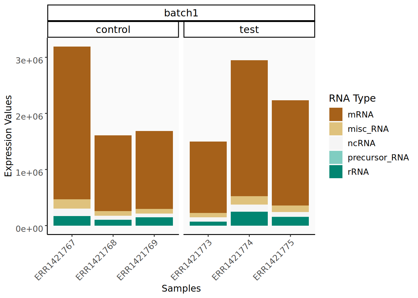
Filtering
You can filter the expression data based on annotation criteria.
Filtering by Annotation
Use $filter_and_set_selected_ids() to keep or exclude expression tags based on their annotation (e.g., keep only mRNAs from a specific species). Filters are applied sequentially (intersecting results). Use $reset() to clear filters.
Code
# Example: Keep only 'mRNA' type transcripts
expr_tx$filter_and_set_selected_ids("mRNA", "type")
# Example: Keep only 'Homo sapiens' transcripts (assuming this is the species)
expr_tx$filter_and_set_selected_ids("Homo sapiens", "tax_name")
# Show summary again to see the effect of filtering
expr_tx$show_etags_summary()
$tax_id ERR1421767 ERR1421768 ERR1421769 ERR1421773 ERR1421774 ERR1421775 9606 2720855 1352015 1389538 1273010 2426011 1877701
$tax_name ERR1421767 ERR1421768 ERR1421769 ERR1421773 ERR1421774 ERR1421775 Homo sapiens 2720855 1352015 1389538 1273010 2426011 1877701
$type ERR1421767 ERR1421768 ERR1421769 ERR1421773 ERR1421774 ERR1421775 mRNA 2720855 1352015 1389538 1273010 2426011 1877701
Refer to ExprData for more filtering options and other methods.
Summarize at the Gene Level
Often, analysis is performed at the gene level. ExprDataGene aggregates transcript-level data.
Initialization (ExprDataGene)
Create an ExprDataGene object from an ExprDataTranscript object. It sums transcript counts to the gene level and calculates weighted average lengths.
Code
# Example: Creating a gene-level expression data object from the transcript-level one
expr_gene <- nexodiff::ExprDataGene$new(expr_tx)
# Show summary at the gene level
p <- expr_gene$plot_etags_summary()
Distributions of types
Code
p$tax_name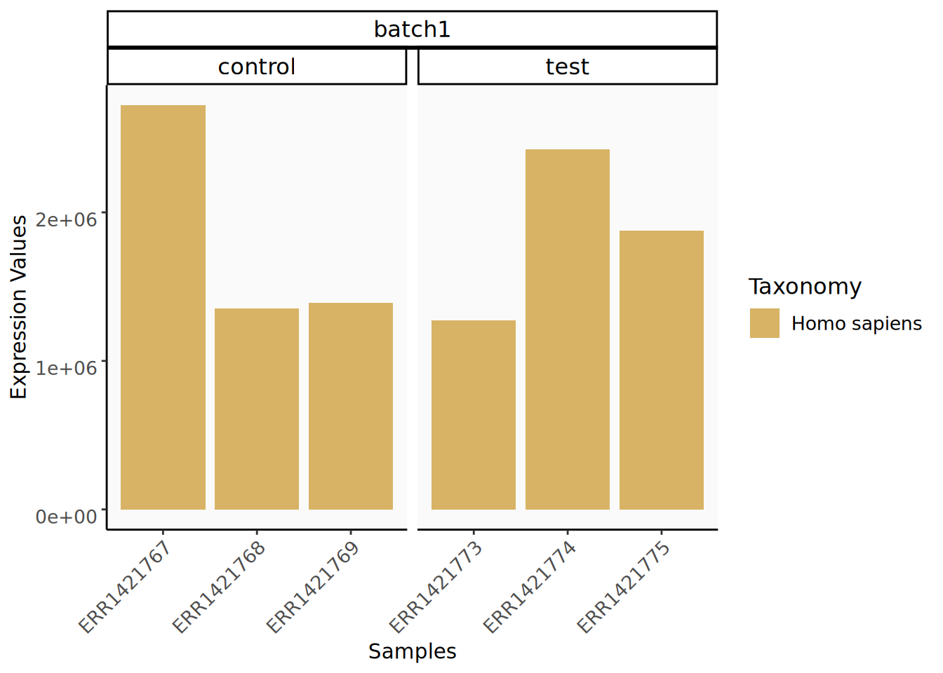
Code
p$type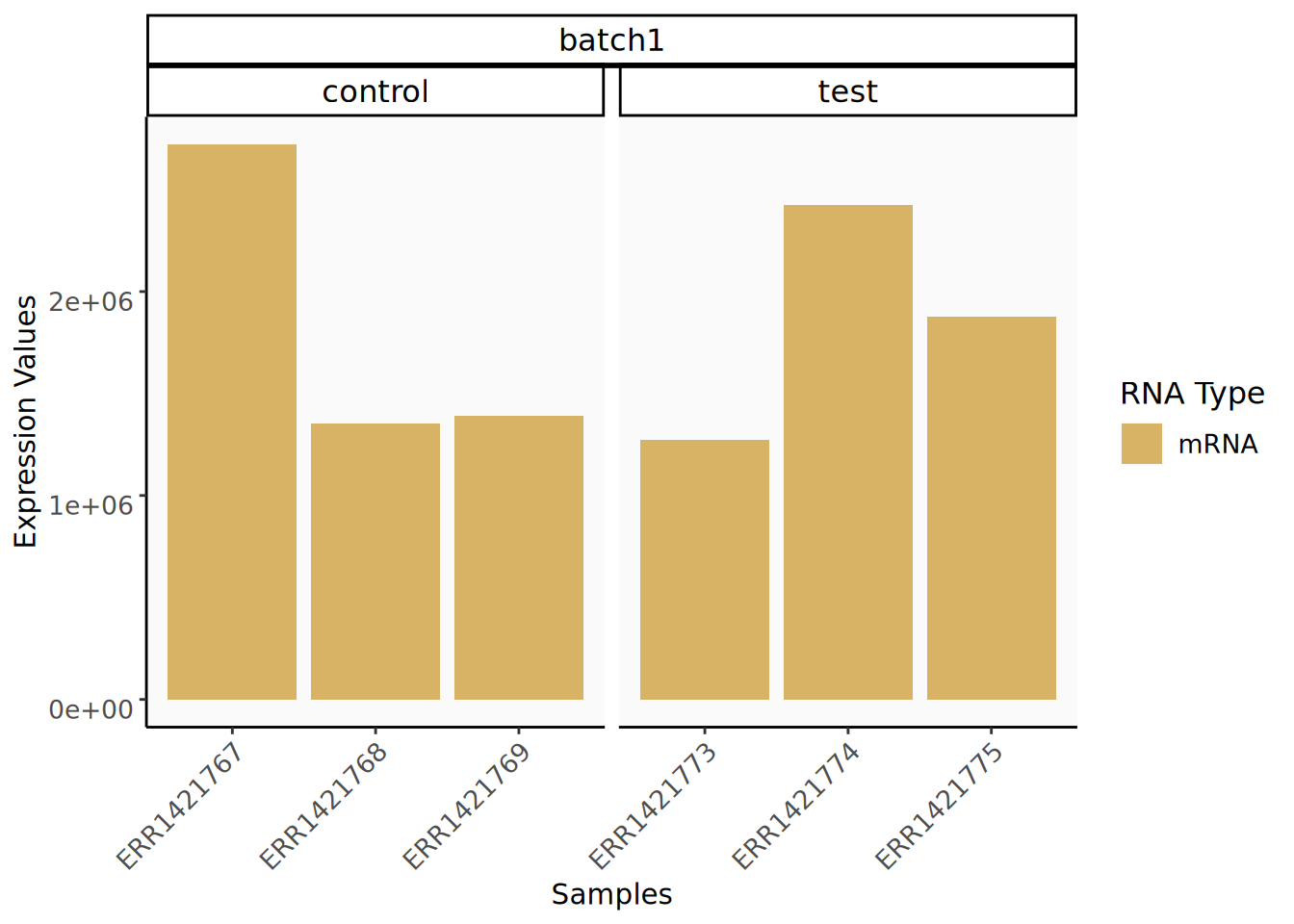
Normalization
Normalization adjusts raw counts for sequencing depth and other factors. nexodiff supports both intra-sample and inter-sample normalization.
Intra-sample Normalization
This adjusts for factors like transcript length within a single sample. Common methods include TPM, FPKM, etc.
Code
# Example: Apply TPM normalization (Transcript Per Million)
# This calculates and stores the intra-normalization factors internally
expr_gene$compute_and_set_intra_norm_fact(method = "tpm")
# Note: Use expr_tx for transcript-level normalization if needed before gene summary
Inter-sample Normalization
This adjusts for differences in library size or composition between samples, making them comparable. Methods like Median Ratio or TMM are common.
Code
# Example: Apply Median Ratio normalization across groups within batches
# This calculates and stores the inter-normalization factors internally
expr_gene$compute_and_set_inter_norm_fact()
Refer to ExprData documentation for details on normalization methods and options.
Quality Control Plots
Visualizing the data is crucial for quality control. ExprData provides several plotting functions.
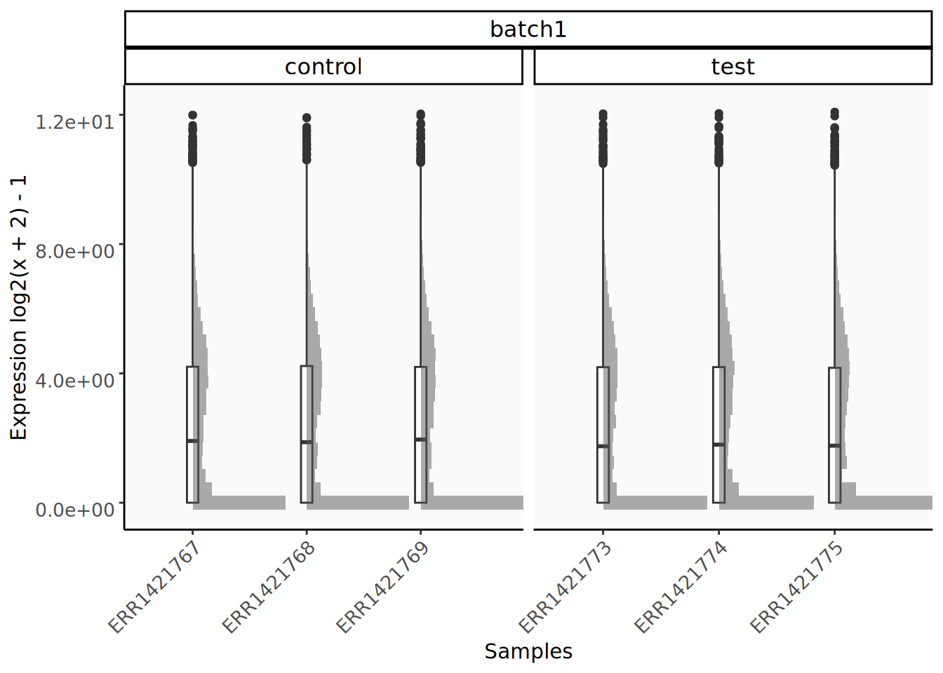
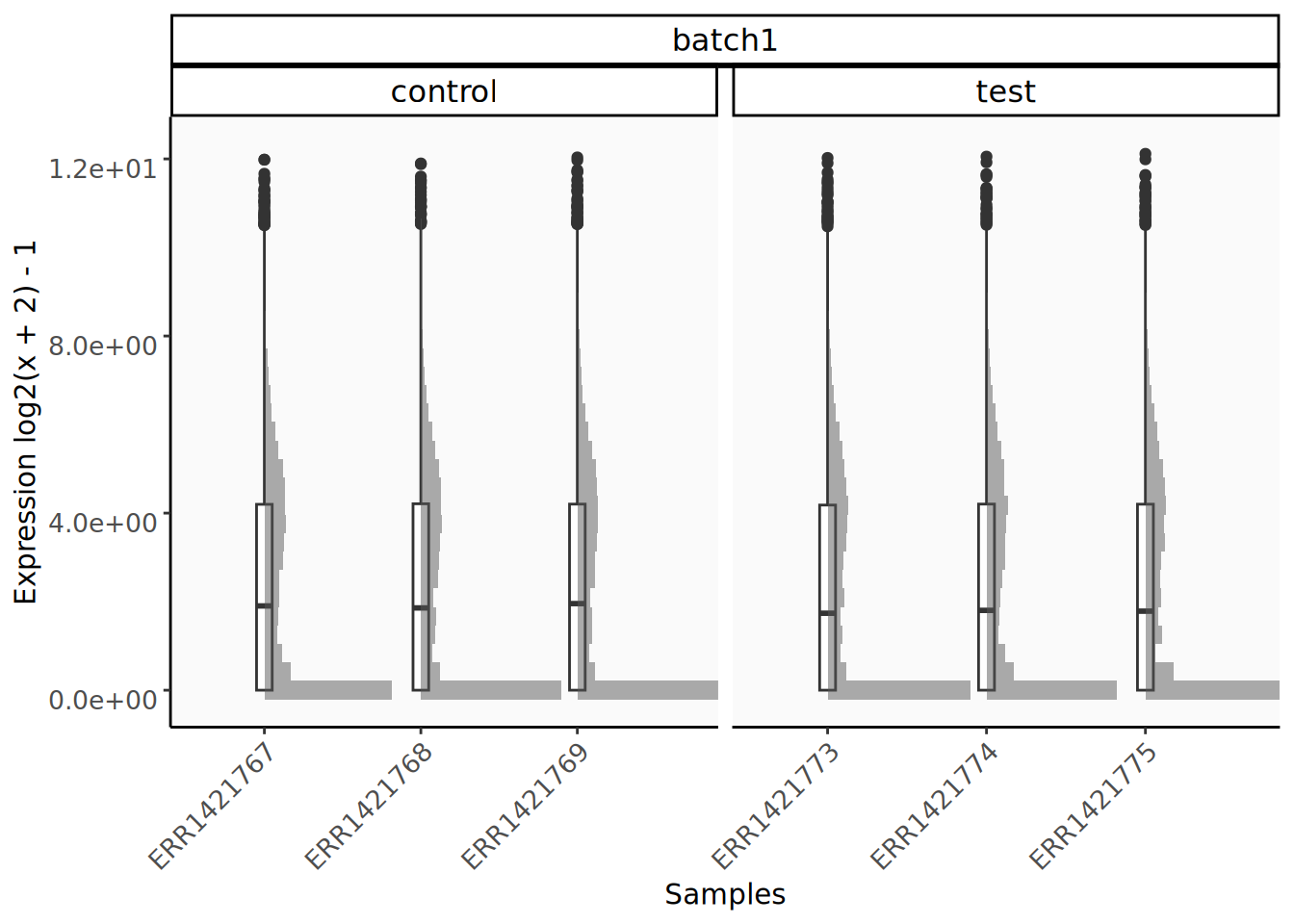
Sample Distributions
Plot the distribution of expression values (raw or normalized) for each sample.
Code
# Example: Boxplot of log2(TPM + 2) expression values per sample
expr_gene$plot_dist_per_sample(
  intra_norm = TRUE,
  inter_norm = FALSE
)
Code
# Example: Boxplot of log2(TPM + 2) expression values per sample
expr_gene$plot_dist_per_sample(
  intra_norm = TRUE,
  inter_norm = TRUE
)
Principal Component Analysis (PCA)
PCA helps visualize the main sources of variation in the data and identify sample clustering or outliers.
Code
expr_gene$plot_prcomp(plot_scale = "design")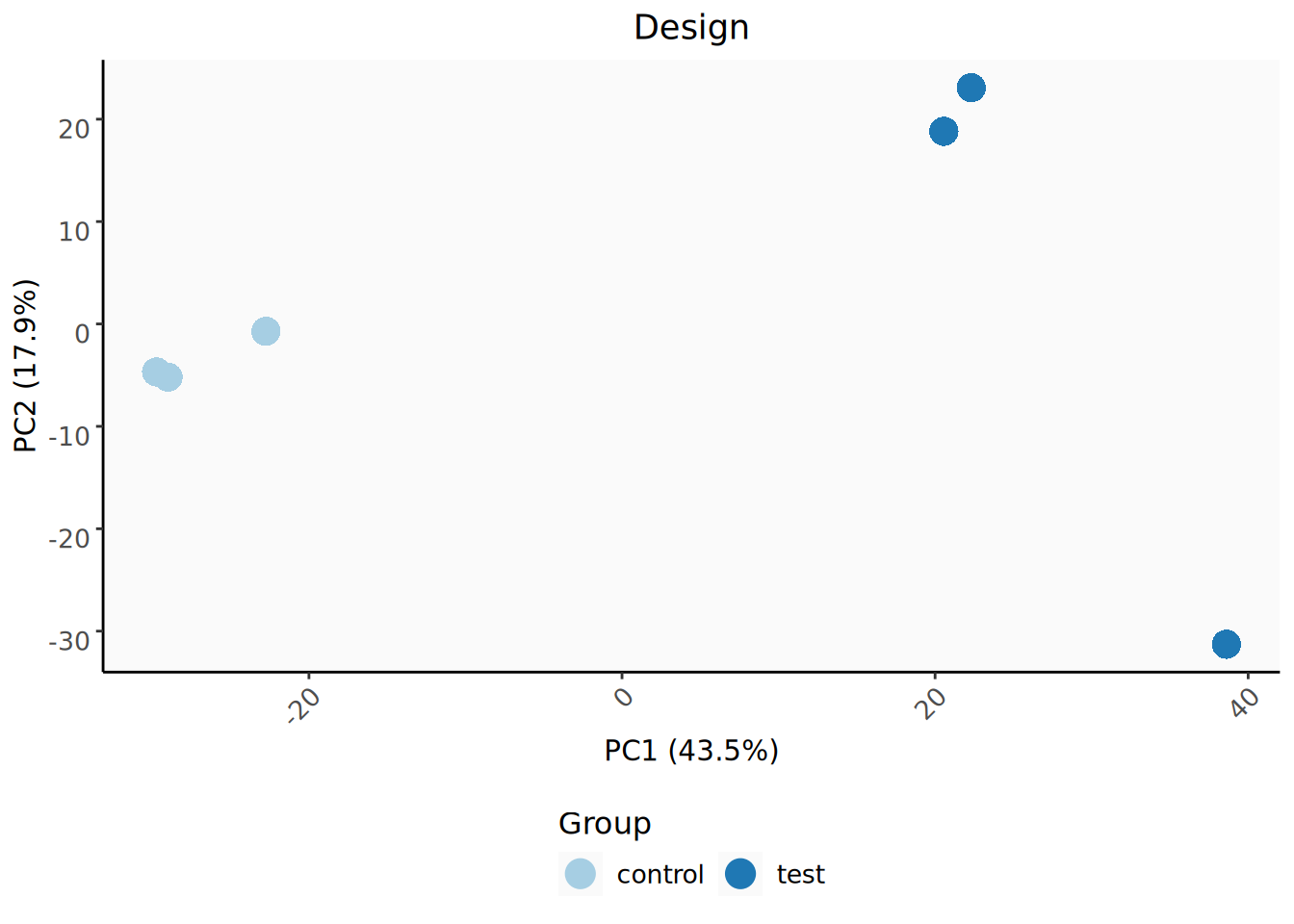
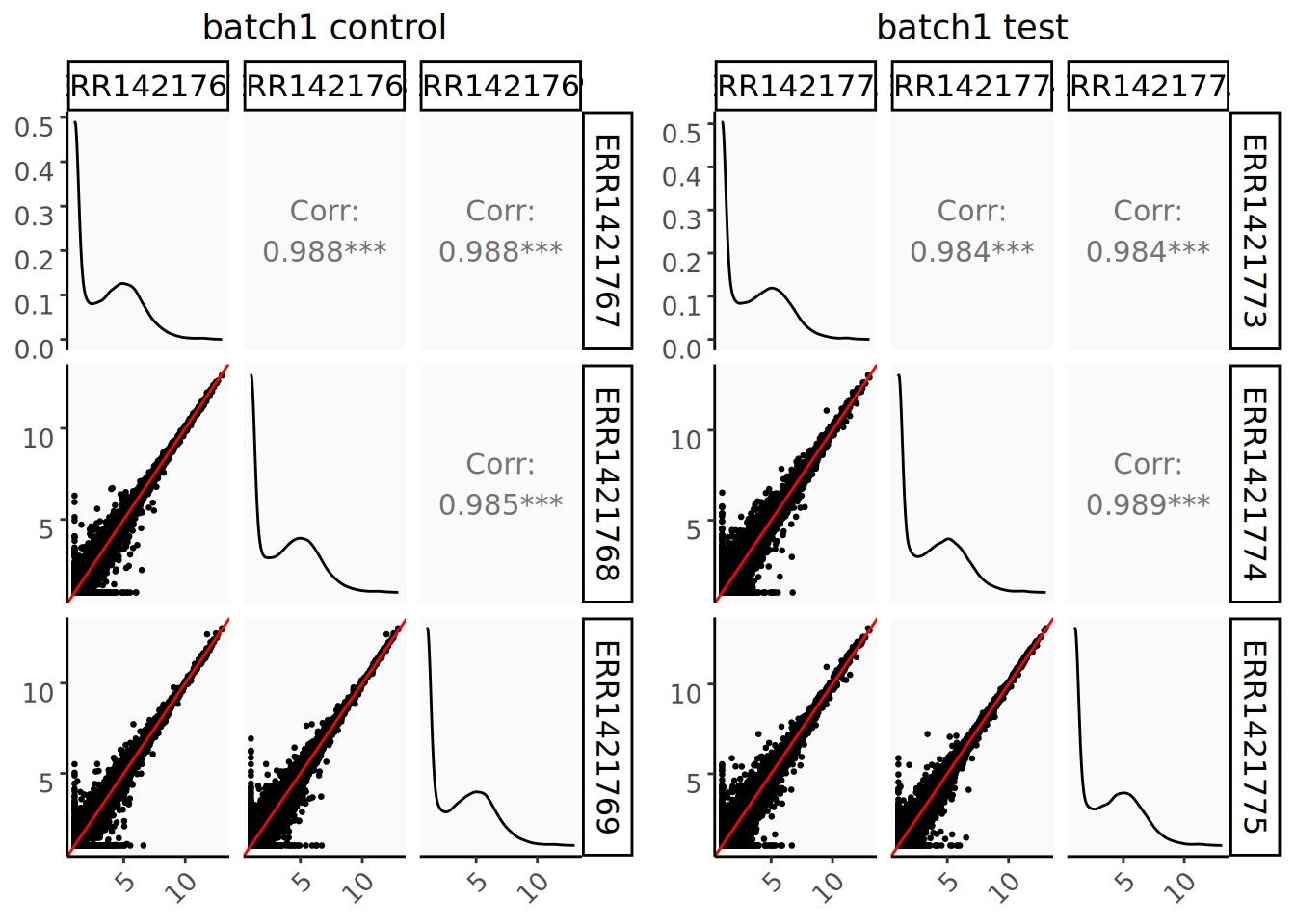
Correlation Heatmap
Assess sample-to-sample similarity using correlation.
Code
expr_gene$plot_corr(
  intra_norm = TRUE,
  inter_norm = TRUE,
  tr_fn = function(x) log2(x + 2)
)
Refer to ExprData documentation for more plotting options and customizations.
Differential Expression Analysis
The core analysis involves identifying differentially expressed genes/transcripts between conditions. nexodiff provides several classes for this, inheriting from PairwiseComp.
Using DESeq2 (PairwiseDESeq2)
Integrates the popular DESeq2 method for differential expression analysis.
Code
# Example: Perform DESeq2 analysis on the gene-level data
# Assumes expr_gene has appropriate normalization factors set or uses DESeq2's internal normalization
pairwise_deseq2 <- nexodiff::PairwiseDESeq2$new(
  expr_data = expr_gene,
  ncpus = 2 # Specify number of CPUs if desired
)

# Explore results (example: get results table for a specific comparison)
# results_df <- pairwise_deseq2$filter_and_get_results(in_batch = "batch1", in_group = "groupA")
# pairwise_deseq2$plot_vulcano(in_batch = "batch1", in_group = "groupA")
Exploring Differential Expression Results
Once you have run a differential expression analysis (e.g., using PairwiseDESeq2), you can explore the results in various ways. The following examples use the pairwise_deseq2 object created earlier.
Getting Results Tables
Use $filter_and_get_results() to extract the results table for specific comparisons, optionally adding annotation columns.
Code
# Example: Get DESeq2 results for group 'groupA' in batch 'batch1'
# (replace with actual group/batch names from your design)
# Add gene symbol and protein names to the table
results_df <- pairwise_deseq2$filter_and_get_results(
    in_batch = "batch1",
    in_group = "test",
    add_ids = c("symbol", "protein_names")
  )
knitr::kable(head(results_df))| batch | group | baseMean | log2FoldChange | lfcSE | pvalue | padj | status | tgid | n_test | n_ctrl | symbol | protein_names |
|---|---|---|---|---|---|---|---|---|---|---|---|---|
| batch1 | test | 227.8372 | -2.595544 | 0.1518830 | 0 | 0 | analyzed | 23435_mRNA | 3 | 3 | TARDBP | TAR DNA-binding protein 43 (TDP-43) |
| batch1 | test | 217.9952 | -2.038275 | 0.1376715 | 0 | 0 | analyzed | 5214_mRNA | 3 | 3 | PFKP | ATP-dependent 6-phosphofructokinase, platelet type (ATP-PFK) (PFK-P) (EC 2.7.1.11) (6-phosphofructokinase type C) (Phosphofructo-1-kinase isozyme C) (PFK-C) (Phosphohexokinase) |
| batch1 | test | 186.4592 | -2.222909 | 0.1512401 | 0 | 0 | analyzed | 22919_mRNA | 3 | 3 | MAPRE1 | Microtubule-associated protein RP/EB family member 1 (APC-binding protein EB1) (End-binding protein 1) (EB1) |
| batch1 | test | 830.5852 | -1.145329 | 0.0784648 | 0 | 0 | analyzed | 6319_mRNA | 3 | 3 | SCD | Stearoyl-CoA desaturase (hSCD1) (EC 1.14.19.1) (Acyl-CoA desaturase) (Delta(9)-desaturase) (Delta-9 desaturase) (Fatty acid desaturase) |
| batch1 | test | 177.0111 | 2.220135 | 0.1555062 | 0 | 0 | analyzed | 127933_mRNA | 3 | 3 | UHMK1 | Serine/threonine-protein kinase Kist (EC 2.7.11.1) (Kinase interacting with stathmin) (PAM COOH-terminal interactor protein 2) (P-CIP2) (U2AF homology motif kinase 1) |
| batch1 | test | 231.9575 | -1.777460 | 0.1338446 | 0 | 0 | analyzed | 54918_mRNA | 3 | 3 | CMTM6 | CKLF-like MARVEL transmembrane domain-containing protein 6 (Chemokine-like factor superfamily member 6) |
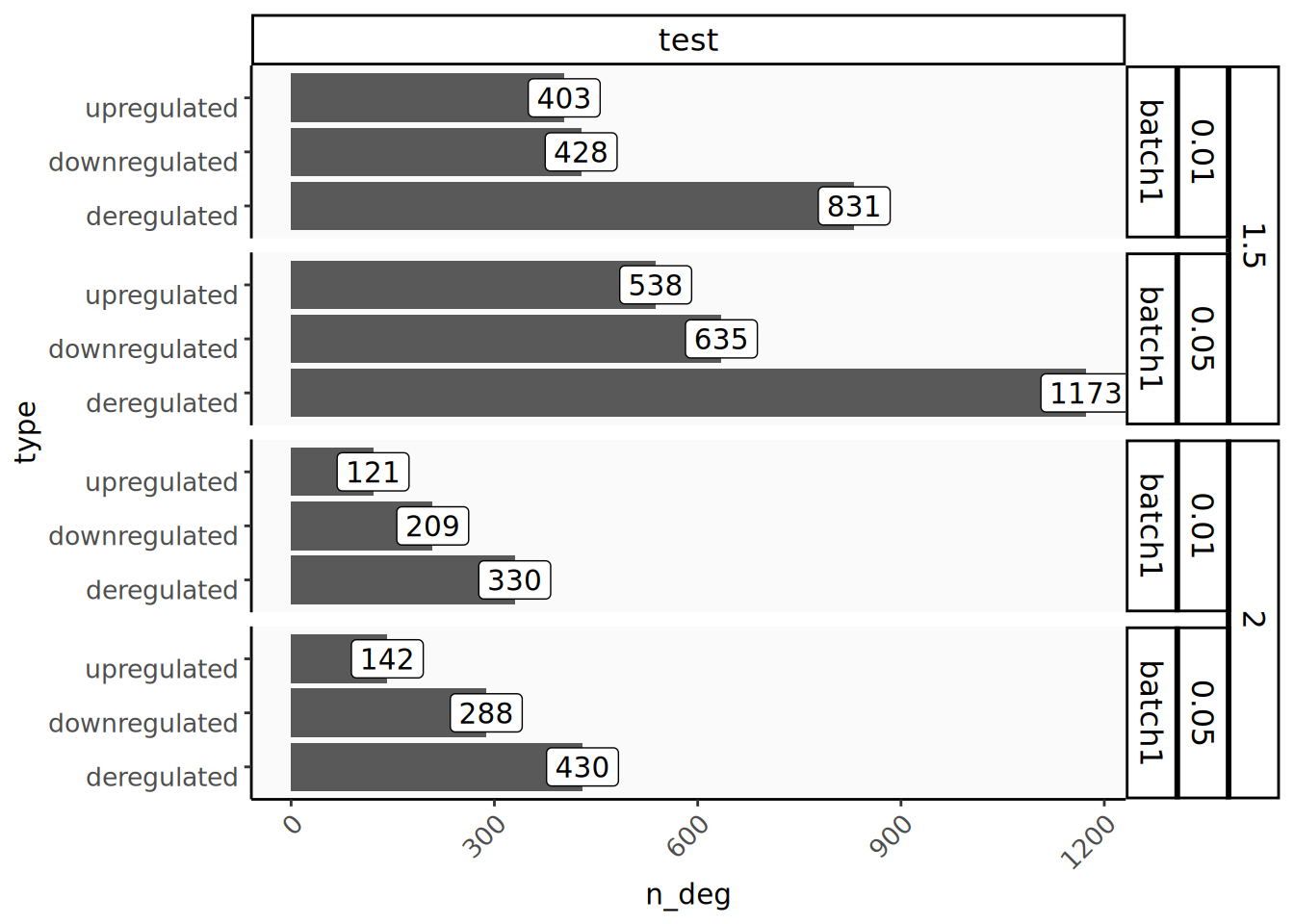
Summarizing Results
Generate a summary table counting the number of differentially expressed genes based on different criteria (LFC, p-value).
Code
# Example: Generate a summary of deregulated genes using different thresholds
summary_df <- pairwise_deseq2$generate_summary(
  cross_id = c("symbol", "uniprot"),
  cross_type = c("deregulated", "upregulated","downregulated"),
  cross_lfc_abs_lim = c(log2(1.5), 1),
  cross_min_signif = c(0.01, 0.05),
  use_padj = TRUE
)


knitr::kable(summary_df)| batch | group | lfc_abs_lim | min_signif | type | n_deg |
|---|---|---|---|---|---|
| batch1 | test | 0.5849625 | 0.01 | deregulated | 831 |
| batch1 | test | 0.5849625 | 0.01 | upregulated | 403 |
| batch1 | test | 0.5849625 | 0.01 | downregulated | 428 |
| batch1 | test | 1.0000000 | 0.01 | deregulated | 330 |
| batch1 | test | 1.0000000 | 0.01 | upregulated | 121 |
| batch1 | test | 1.0000000 | 0.01 | downregulated | 209 |
| batch1 | test | 0.5849625 | 0.05 | deregulated | 1173 |
| batch1 | test | 0.5849625 | 0.05 | upregulated | 538 |
| batch1 | test | 0.5849625 | 0.05 | downregulated | 635 |
| batch1 | test | 1.0000000 | 0.05 | deregulated | 430 |
| batch1 | test | 1.0000000 | 0.05 | upregulated | 142 |
| batch1 | test | 1.0000000 | 0.05 | downregulated | 288 |
Code
Plotting Results
Visualize the results using standard plots.
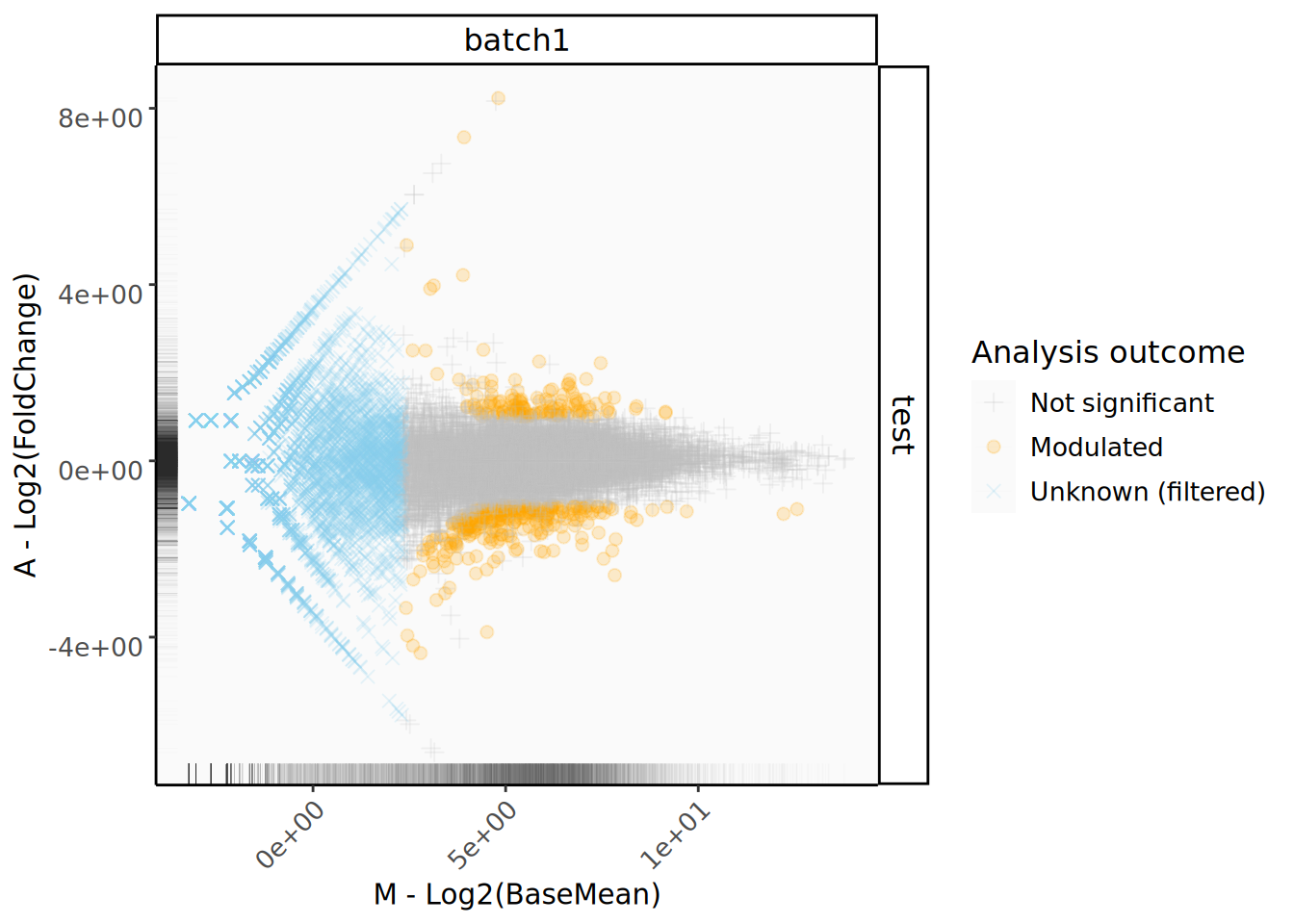
MA Plot
Shows log2 fold change versus mean normalized counts. Useful for visualizing magnitude of change and identifying potential biases.
Code
# Example: MA plot for a specific comparison
pairwise_deseq2$plot_ma(
  lfc_abs_lim = 1,      # LFC threshold for coloring
  min_signif = 0.05,    # Significance threshold for coloring
  use_padj = TRUE
)
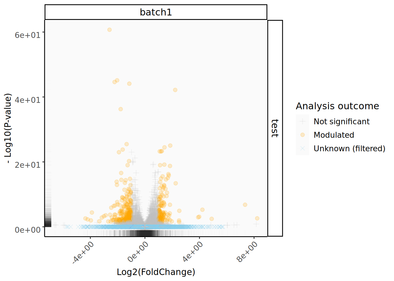
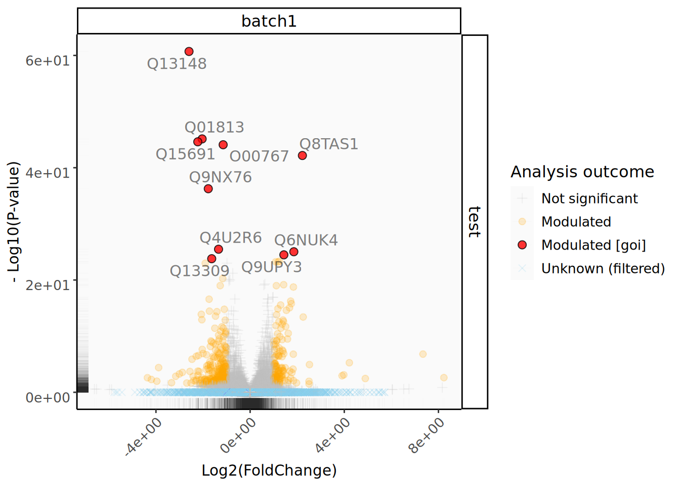
Volcano Plot
Plots statistical significance (-log10 p-value) versus log2 fold change. Helps identify statistically significant genes with large magnitude changes.
Code
# Example: Volcano plot for a specific comparison
pairwise_deseq2$plot_vulcano(
  lfc_abs_lim = 1,      # LFC threshold for coloring/lines
  min_signif = 0.05,    # Significance threshold for coloring/lines
  use_padj = TRUE,
)
Code
# Example: Volcano plot for a specific comparison
pairwise_deseq2$plot_vulcano(
  lfc_abs_lim = 1,      # LFC threshold for coloring/lines
  min_signif = 0.05,    # Significance threshold for coloring/lines
  select_ids = pairwise_deseq2$generate_a_list(in_batch = "batch1", in_group ="test", id = "uniprot")[1:10],
  tag_id_select = "uniprot",
  tag_id_show = "uniprot",
  use_padj = TRUE,
)
Heatmap
Visualize the expression patterns of selected genes across samples.
Code
# Example: Heatmap of top differentially expressed genes

pairwise_deseq2$plot_heatmap(
  lfc_abs_lim = 1,
  min_signif = 0.05,
  use_padj = TRUE,
  select_ids = pairwise_deseq2$generate_a_list(in_batch = "batch1", in_group ="test", id = "tgid", top_x = 100),
  tag_id_select = "tgid",
  tag_id_show = "symbol",
  max_tags = 500,
  hard_select = TRUE
)
2026-03-25 14:14:30.95478 WARNING::max_tags > 15 is not ideal for visibility clust
Call: hclust(d = tag_dist, method = meth_clust)
Cluster method : centroid Distance : minkowski Number of objects: 100
Refer to PairwiseComp documentation for many more plotting options and customizations.
Exporting Results
You can easily export the differential expression results to an Excel file, with each sheet representing a comparison (group within a batch).
Code
# Example: Write results for all comparisons to an Excel file
pairwise_deseq2$write_to_xlsx(
  output_folder = ".", # Save in the current directory
  file_suffix = "_deseq2_results.xlsx"
)
This concludes the basic workflow using nexodiff. Explore the detailed documentation for each class to understand all available parameters and advanced features.